Difficulties of Language Modelling and it's approximations
Language model is a parameterised probability function $P(x;\theta)$ which takes a sentence as an input ‘x’ and evaluates how probable the given sentence is. Given the entire corpus of english vocabulary, our goal is to learn a good probabilistic model i.e. learn the parameters $\theta$ such that it outputs a high probability value for a well formed sentence and low probability value for a grammatically incorrect sentence
This blog tries to quickly go over through the probabilistic formulation of a Language model, the difficulties in learning a model and how can we confront them with approximations having theoretical guarantees.
The post follows the following topics in sequence:
- Lang model formulation and Initial approaches
- Problems with initial approaches and Curse of dimensionality
- Neural network as a smooth continuous density function
- Partition function complexity
- Noise Constrastive Estimation(NCE) to side-step Partition function
- Adapting NCE for Lang models
Lang Model Formulation
The role of language model is to estimate likelihoods of sequence of words or the next word given a history sequence, both the same. Each word in a sentence is a discrete Random Variable with a domain of the size of Vocabulary ‘V’, so the joint-distribution of a length ‘k’ sentence will have $|V|^k$ parameters(table entries) - a parameter blowup :Curse of dimensionality. For those of us who have seen Bayesian networks, the next logical step would be to use the chain rule to divide the joint probability model into factors and assume few conditional independencies.
Let’s first factorise: $ P(w_1,w_2,…w_k) = P(w_1)*P(w_2|w_1)*P(w_3|w_{1:2})…P(w_k|w_{1:k-1}) $
Each of the factor is probability of a word given it’s history: $P(w \vert h)$. One way to estimate this quantity is to take the relative frequency counts.
Considering the example ‘Amherst almost freezes into ice during winter’, this would be:
As we could clearly observe, the frequency of ‘Amherst almost freezes into ice during’ is very rare and such estimates are not generalizable to new similar sentences having similar syntactice and semantice structures at all. We would have different sentences in training data and test data. A sentence “Amherst Noun freezes into ice during winter” learnt in training data should add probability mass to “Atlantic Noun freezes into into ice during winter” seen in test set.
Now we can introduce ‘Conditional independence’ assumptions to decrease the number of parameters and find a way around achieving generalisability. The n-gram language model dictates that each word depends only the previous n-words. The model approximates $P(w_k \vert w_{1:k-1})$ as $P(wk \vert w_{k-n:k-1})$. Bi-grams(n=2) and Tri-grams(n=3) are traditionally widely used(especially with huge training corpuses) and are used as standard baselines for new language model techniques being introduced. In a bi-gram model, as we could observe, there are many conditional factors in the training example ‘Amherst almost freezes into ice during winter’ which can be reused to predict the probability of ‘Atlantic almost freezes into ice during winter’. This is way of approaching a sequence of words as “gluing” very short and overlapping pieces of length 2 or 3 that have been seen frequently in the training data. Few additional tricks are used in this model to given better performin variants: backoff n-gram model and others. This paper outlines many tricks used along standard n-gram models. For more details and clarity on n-gram models Jurafsky book is a good reference.
Drawbacks
In n-gram language models, we take two strong assumptions which should be addressed upon:
- Temporal dependence: Adopting n-gram conditional independence, we assume that temporally closer words are more statistically dependent and eschew longer contexts and also only depend on LHS words in-order to predict a word.
- Generality in word meanings and their similarity in any abstract level is not being taken into account. This allows us to identify that ‘Amherst’ and ‘Atlantic’ are similar in their grammatical, semantic roles (both are Nouns, Places, located towards the Western hemisphere etc…)
Continous functions
With above lessons learnt, let us not throw away distant words/randomvariables and model them in our distribution model. Let us re-consider our massive Joint Probability table that we have mentioned in the beginning. This parameter blow-up in this model owes to considering each ‘word’ as a discrete random variable and then so to the massive domain size of each random variable- ‘size of the entire Vocabulary’. Continuous probability models with continuous random variables as input, on the other hand, model data distributions with very few parameters. For instance, Normal distribution has just two parameters: Mean, Variance for predicting probabilities for a given real-valued continuous input random variable.
Neural Probabilistic model proposed by Bengio et.al is the continuous counterpart for language models. This model :
- considers each word as a real-valued vector of an assumed dimension ‘d’ (d $\ll \vert V \vert$ - hence avoids the dimensionality problem)
- Models the probability distribution function using a Continuous model like: a plain linear Softmax-regression or a non-linear Neural model. The model $f(\hat{w_1}, \hat{w_2},…\hat{w_k})$ takes the ‘k-1’
d-dimensional word vectors as input to output the probability: $P(w_k \vert w_{1:k-1})$. Here, $\hat{w}$ refers to real valued vector of the word ‘w’.
The learning problem in this model is to learn both the real-valued representations of the words and the model function ‘f’(neural net weights) to maximise the likelihood of the training-data.The feature vectors associated with each word are learned, but they could be initialized using prior knowledge of semantic features(e.g.: GLOVEs)
This model generalises well because similar words have similar real-valued vectors. What ever probability model we are fitting the data with is a continuous function, like neural network or a simple linear softmax-regression model, over these continuous word vectors. Hence small changes in the vectors will lead to small change in probability estimates. Therefore, the presence of only one of the sentences in the training data will increase the probability, not only of that sentence, but also of its combinatorial number of “neighbors” in sentence space (as represented by sequences of word vectors).
While the words(input) are continuous now with similar words being chunked together in the input space, our probability function(Neural network) has to learn from training corpus to put more probability density over these similar chunk of word groupings(structure) which have repeated more often.
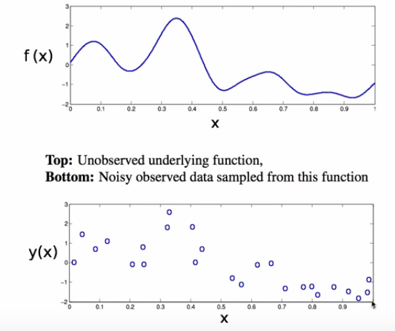
Bengio et. al says and we rephrase that a good generalising language model should not just distribute probability mass uniformly around each training example. This was the case in the discrete joint prob table setup where each word combination entry in the table occupied uniform probability mass. Keeping this in mind and we can motivate the previous two points by comparing our case with the non-parametric density estimation problem setting where the density function is estimated based on the given training examples with out any inductive bias(i.e. no parameters). Here the density is not uniformly distributed around the training example, but is ‘smoothly’ distributed based on a similarity measuring function referred as Kernel function. Following figure is an examples estimating the density of the training data(bottom figure) using Gaussian Kernel to result in density distribution(top half).
Architecture of Neural Lang Models
Widely used Neural language models are not deep like networks used to model Image distributions(but have a lot of parameters). The simplest model used is a Softmax regression model, where given a context sentence(or history), all the word vectors in the context are weighted-summed and the resultant vector is soft-max regressed over the entire vocabulary-set to know how much each words in the vocabulary is probable. It is a linear regression over the semantic word vector space and does not have non-linearities. This simple linear model is also referred as log-bilinear model. Even this simple linear model which can be summed up with the two below equations has been shown to outperform the aforementioned n-gram model.
For those who are aware of word-embedding training models like Skipgram, the $\hat{w_i}$ is refered as input word embedding representation and $q_w$ is referred as the target(output) embedding representation. We are multiplying these two vector representations to get a score metric and hence the name ‘bilinear model’. Multiplying two different vector spaces is referred as BiLinear multiplication. The position dependent context weights ‘C_i’ can be fixed to ‘1’ for a naive start. Just as an interesting addition, this paper mentions that ‘b_w’ acts a parameter which would model the popularity or frequency of the word ‘w’.
The major chunk of parameters in neural language models is taken by the word vector representations. So we can say that the memory complexity of the neural language model is linear in the vocabulary size. OTOH, n-gram models are linear in the training set size. This is a very reasonable saving. However, the training time of this neural language model is going to be significant. The major bottleneck being the softmax regression at the last step of the model where the input representations are projected over the entire vocabulary of words and softmax-normalised. If ‘d’ represents the word-vector dimension, this softmax regression takes V*d operations. And this is done for every training example which slows down our entire training pipeline. Below we will introduce a technique called Noise Contrastive Estimation and later explain how this techniques can be applied to our setting to allieviate this problem.
Noise Constrastive Estimation:
Given the job of computing a probability density function say $P_m(\theta)$, NCE is a technique which modifies this objective into an easier objective which can sidestep the normalisation computation. The main intuitive idea in NCE is estimate a target density function($P_m$) relatively, using a noise distribution. An analogy would be to estimate the area of the waterscape on earth by relatively saying everything which is not a land mass is a water body. Here if we know the landmass density, we can figure out the water bodies density. We introduce an additional density distribution in NCE which is referred as ‘noise’ just like how we have introduced ‘land masses’ in our analogy to estimate water bodies. This noise-distribution is a known distribution just like how we assumed we know the landmass density. Note: Let this example not bias us to think that Noise and True distributions are complements. It is not a requirement. For the sake of an easy understanding example, the two entities are disjoint and the relation between the distributions is complementary, but however this analogy is not fully representative.
Let $X = \{ x_1,x_2,….x_{Td} \}$ represent the given sample data of a random variable ‘x’ drawn from a probability density distribution $p_d$, which we aim to figure out. As we would normally assume in a parametric modelling case, let ‘pd’ be a member of the parametric family of the distribution $p_m(X;\theta)$ i.e. there exists $\theta^*$ such that $p_d = p_m(X;\theta^\ast)$.
Now consider a known distribution $p_n$ used as our Noise distribution and let $Y=\{y_1,y_2….,y_{Tn}\}$ be the sample from $p_n$.
Now we are going to create a mixture of data $U = X \cup Y = \{u_1, u_2, …, u_T\}$. Each of the $u_i$ is either from the noise(C=0) or from the unknown distribution we want to findout $p_m$ (C=0). It is a classic supervised classification problem to learn to distinguish between these two classes.
Priors are:
Class Posteriors are:
where $k=\frac{Tn}{Td}$ is nothing but how many noise samples do we have for each true sample
Since the random variable ‘C’ is bernoulli and if the data samples in ‘U’ are assumed to be IID, the conditional likelihood is given by:
Dividing by $Td$ doesnt change the optimisation problem but helps us characterize the objective function using weak law of large numbers
We can discover now that optimizing $l(\theta)$ leads to an estimate $\theta_{1}$. But is this estimate $\theta^{1}$ equal to our required estimate $\theta^{*}$?– It is so and we will talk about how it is soon.
Role of ‘k’:
The gradient of eq-3 would be equal to : (Note the form in terms of $log(P_m(u;\theta))$)
Resolving the expectation, the above gradient can be written as:
As $k \to \infty:\quad \frac{\partial}{\partial \theta}l(\theta)=\sum_u\left(P_d(u)-P_m(u;\theta)\right)*\frac{\partial}{\partial \theta}lnP_m(u;\theta)$
If you are familiar with softmax-crossentropy function derivative, it can be observed the above equation is in the same form and hence we can say as ‘k’ increases, the NCE objective gradient converges with the cross-entropy used MLE objective gradient. However, in practical we wouldnot want to choose large ‘k’ values and bring in the computational complexity to our training pipeline. It has been emperically shown that the value of ‘k’ and the mutual-information between noise($P_n$), true($P_m$) distributions have a relation. This paper shows that using Unigram distribution as $P_n$ needs ‘k’ value as 25 to perform equivalent to MLE and using Uniform distribution as noise needs very high ‘k’ values to converge.
Treating Normalisation function as a parameter
We have seen that by solving the given binary classification objective we estimate the initial unsupervised density estimation objective. But till now $p_m$ was still assumed as proper PDF satisfying the normalisation axiom i.e. the complexity of Normaliser computation is still present eventhough we have transformed our objective. Extending this idea to unnormalised distributions say $p_m^0$ is the main genius of NCE.
Restating our goal specifically, we want to estimate a $\theta^{\ast}$ to find a valid PDF such that the basic two probability axioms are satisfied: Normalisation Constraint and Positivity constraint Normalisation constraint: $\int p_m(u;\theta)du=1$ A model is innately normalised when any value of $\theta$ used in the model satisfies the above two constraints. Our previous mentioned Neural language model is one such owing to the softmax at the end. This is the typical case in most ML settings where we can use MLE to estimate $\theta^*$. However, our goal is to remove the end Softmax layer and maximise using unnormalised distribution say $P_m^0(;\alpha)$. As we know, this unnormalized model can be normalised by dividing by its normaliser, but we dont want to compute it but estimate it. NCE just does that by introducing the Normaliser as a parameter into the model along with $\alpha$ parameter set. Now all $P_m(u;\theta)$ will be written in form of ${P_m^{0}(u;\alpha)\ast 1/z}$.
Maximizing this objective will be estimate the approximate the ‘z’ term and converges to the actual normalization term as Td increases to $\inf$. A fundamental point in the theorem is that the maximization is performed without any normalization constraint. With the NCE objective function, no such constraints are necessary. The maximizing pdf is found to have unit integral automatically. It can be proved that the landscape of this objective function has a single extrema(and that it is maximum) and the extremum happens at a $\theta$ where $P_m(\theta) =P_d$; Proof in Appendix A.2. That means the converged extremum is a valid PDF which will have a normaliser parameter respecting the Normalisation axiom.
Putting NCE to work in Lang Modelling setting
In our training pipeline, for a given example context:next_word pair:(w, h), the objective gradient is computed as:
Where $n_i$ refers to ith noise sample.
The gradient is still kept in normalised form $P_m(w; \theta, h)$ instead of writing in terms of its unnormalised form. We will address this shortly.
For each context ‘h’, we will have a different a different distribution $P_m(w; \theta, h)$ i.e. different score distributions $score_{\alpha}(w, h) \; \text{and} \; z$. So each context ‘h’ needs a separate ‘z’ to be stored. What this paper discovered is if ‘z’ parameter is fixed as ‘1’ the performance wouldnt
be affected much. Since there were a lot of parameters in the model, fixing the normaliser to ‘1’ forced the scores to converge to valid probabilities.
The objective gradient for a given (w, h) would then be just:
Refer the mentioned paper for more context on the experiments run and the results obtained.
The computational savings made using this technique from the final softmax regression is from $\vert d\ast V\vert$ to $\vert d\ast k\vert$
REFERENCS:
N-gram improvement tricks: https://arxiv.org/abs/cs/0108005
N-gram Language models: https://web.stanford.edu/~jurafsky/slp3/4.pdf
Probabilistic Neural Language model: http://www.jmlr.org/papers/v3/bengio03a.html
Noise Constrastive Estimation : http://www.jmlr.org/papers/v13/gutmann12a.html
NCE for Language modelling: https://www.cs.toronto.edu/~amnih/papers/ncelm.pdf